Scilab - 查找巴特沃斯系数并过滤模拟数据

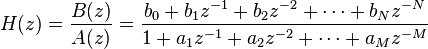
如何解决Scilab - 查找巴特沃斯系数并过滤模拟数据

对于带有加速度计的项目，我正在寻找一种过滤高频的方法。我不是信号专家，但我通常是根据我的需要阅读的，使用了巴特沃斯滤波器。

我为此目的使用 Scilab，我正在努力解释我的结果：我编写了以下代码（底部）并比较了 Scilab 输出函数以在 Arduino 中实现此 filtering equation :>

我的问题是：

cnum 函数和过滤器函数有什么区别？
analpf(butt) 或 zpbutt 的结果系数是

"系数：Num / Den："
1.

0.063662 0.0020264 0.0000323

我期望结果为 canonical form 期望值为

b1 0.331785003 ; b2 0.99535501 ; b3 0.99535501 ; b4 0.331785003
a1 -0.965826145 ; a2 -0.582614466 ; a3 -0.106171201

从此处的外部软件 (link) 计算得出，N=3，低通，Fc=5，Fs=15。

你能看看我的代码并给我一些建议来纠正它并获得正确的系数 ai 和 bi 吗？

/////////////////// cleanup
clear;
//clc;
close;


////////////////////// variable declaration
fcut = 5; //cut off frequency hz (delta 1)
fsampl = 15 ; //sampling frequency hz (delta 2)
delta1_in_dB = -3; // attenuation value at fcut
delta2_in_dB = -21; // final attenuation
delta1 = 10^(delta1_in_dB/20)
delta2 = 10^(delta2_in_dB/20)
epsilon = 0; //ripple value [0 1]
rp = [epsilon epsilon] // ripple vector for analpf 

// conversion of attenuation
delta1 = 10^(delta1_in_dB/20);
delta2 = 10^(delta2_in_dB/20);

// N computation
N = log10((1/(delta2^2))-1)/(2*log10(fspan/fcut));
N = ceil(N);
disp("Order",N);

/////////////////// compute different functions to compaire Butterworth
[poleZP,gainZP]=zpbutt(N,fcut*2*%pi);

[hsAna,poleAna,zeroAna,gainAna]=analpf(N,'butt',rp,fcut*2*%pi);

//disp("Pole : Zpbutt ",poleZP,"Analpf ",poleAna)
//disp("Gain : Zpbutt ",gainZP,gainAna)
//disp("function :",hsAna)
//       conclusion : zpbutt et analpf donnent la même sortie

/////////////////// paramters in linear system
// Generate the equivalent linear system of the filter
num   = gainAna * real(poly(zeroAna,'s'));
den   = real(poly(poleAna,'s'));
elatf = syslin('c',num,den);

Cnum=coeff(num);
Cden=coeff(den)/Cnum;
Cnum=1;

disp('coefficients : Num / Den : ',Cnum,Cden)





/////////////////// plot an exemple to compare csim and filter
rand('normal');
Input = rand(1,1000); // Produce a random gaussian noise
t     = 1:1000;
t     = t*0.01; // Convert sample index into time steps

y_csim = csim(Input,t,elatf); // Filter the signal with csim
y_res = filter(Cnum,Cden,Input) // Filter the signal with filter


// plot curves
subplot(3,1,1);
plot(t,Input);
xtitle('The gaussian noise','t','y');
subplot(3,2);
plot(t,y_csim,'b');
xtitle('The ''csim'' filtered gaussian noise',3);
plot(t,y_res,'r');
xtitle('The ''filter'' filtered gaussian noise','y');

提前感谢您的支持！！

解决方法

在将该网站的输出转换为规范形式时，您似乎错过了符号反转。

该网站的输出是：

3.014⋅yi = (1⋅xi + 3⋅xi-1 + 3⋅xi-2 + 1⋅xi-3) + -2.911⋅yi-1 + -1.756⋅yi-2 + -0.320⋅yi-3

当我将其转换为规范形式时，我得到：

yi   (0.331785 + 0.995355*z^-1 + 0.995355*z^-2 + 0.331785*z^-3)
-- = -----------------------------------------------------------
xi      (1 + 0.96582*z^-1 + 0.582614*z^-2 + 0.10617*z^-3)

这意味着：

[b0..b3] = [0.331785   0.99535501 0.99535501 0.331785  ]
[1 a1..a3] = [1.         0.96582614 0.58261447 0.1061712 ]

在 scilab 中获得相同答案的一种简单方法是使用他们的 iir 滤波器设计函数，该函数一步完成模拟设计和双线性变换，如下所示：

--> hz=iir(N,'lp','butt',5./15.,[0 0])
 hz  = 

                                                    
   0.3318051 +0.9954154z +0.9954154z² +0.3318051z³  
   -----------------------------------------------  
       0.1060171 +0.5826442z +0.9657797z² +z³

你可能会说系数向后看，但一定要注意 z 的幂的符号；相对于您希望拥有的规范形式，整个方程已乘以 z³/z³。解决这个问题的简单方法就是获取系数和 flip them from left to right。

--> coeff(hz.num)(:,$:-1:1)
 ans  =

   0.3318051   0.9954154   0.9954154   0.3318051

--> coeff(hz.den)(:,$:-1:1)
 ans  =

   1.   0.9657797   0.5826442   0.1060171

这是我更新后的代码，其中包含@Mark H 提出的解决方案（再次感谢！）。我还有一些问号，主要是面向Scilab的，如果有人可以教我（但这不是我项目的障碍）。

flts 和 filter 函数之间有什么区别？我的输出结果与那些函数不同。

代码：

////////////////////// cleanup
clear;
//clc; clear console
close;

////////////////////// variable declaration
fcut = 10000; //cut off frequency hz (delta 1)
fsampl = 100000 ; //sampling frequency hz (delta 2)
delta1_in_dB = -3; // attenuation value at fcut
delta2_in_dB = -21; // final attenuation

// conversion of attenuation
delta1 = 10^(delta1_in_dB/20);
delta2 = 10^(delta2_in_dB/20);

// order N computation
N = log10((1/(delta2^2))-1)/(2*log10(fsampl/fcut));
N = ceil(N);
disp("Order",N);

///////////////////// computer Butterworth transfer function
hz=iir(N,fcut/fsampl,[ ]);

///////////////////////////// extract coefficient from transfer function
num   = coeff(hz(2));
den   = -1*coeff(hz(3));
gain = 1/num(1)

// display value and graph
disp('gain',gain)
disp('''b'' coefficients : num xi',num)
disp('''a'' coefficients : den yi',den(N:-1:1))

[hzm,fr]=frmag(hz,256);
f = scf(0)
plot(fr,hzm)


/////////////////// plot an exemple
rand('normal');
Input = rand(1,1000); // Produce a random gaussian noise
t     = 1:1000;
t     = t*0.01; // Convert sample index into time steps

//Change from transfer function to linear system
    sl= tf2ss(hz)

//Filter the signal
    fs=flts(Input,sl);

// plot curves of raw and filtered data
f = scf(1)
subplot(2,1,1);
plot(t,Input,'b');
xtitle('The gaussian noise','t','y');
subplot(2,2);
plot(t,fs,'r');
xtitle('The filtered gaussian noise','y');




///////////////////// export on CSV
filename = fullfile(TMPDIR,"data_test_filter.csv");
separator = ";"
M = [t' Input' fs']; //data matrix
csvWrite(M,filename,separator);

filename = fullfile(TMPDIR,"coeff.csv");
C = [gain num den(N:-1:1)] ;//coeff matrix
csvWrite(C,separator);


disp("DONE !");

Scilab - 查找巴特沃斯系数并过滤模拟数据

如何解决Scilab - 查找巴特沃斯系数并过滤模拟数据

解决方法

相关推荐