

目录
Pandas 时间序列处理
1 Python 的日期和时间处理
1.1 常用模块
datetime time calendar
- datetime,以毫秒形式存储日期和时间
- datime.timedelta,表示两个 datetime 对象的时间差
- datetime 模块中包含的数据类型
| 类型 | 说明 |
|---|---|
| date | 以公历形式存储日历日期(年、月、日) |
| time | 将时间存储为时、分、秒、毫秒 |
| datetime | 存储日期和时间 |
| timedelta | 表示两个 datetime 值之间的差(日、秒、毫秒) |
1.2 字符串和 datetime 转换
datetime -> str
- str(datetime_obj)
dt_obj = datetime(2019,8,8)
str_obj = str(dt_obj)
print(type(str_obj))
print(str_obj)
<class ‘str‘>
2019-08-08 00:00:00
- datetime.strftime()
str_obj2 = dt_obj.strftime('%d/%m/%Y')
print(str_obj2)
08/08/2019
str -> datetime
- datetime.strptime()
需要指定时间表示的形式
dt_str = '2019-08-8'
dt_obj2 = datetime.strptime(dt_str,'%Y-%m-%d')
print(type(dt_obj2))
print(dt_obj2)
<class ‘datetime.datetime‘>
2019-08-08 00:00:00
- dateutil.parser.parse()
可以解析大部分时间表示形式
from dateutil.parser import parse
dt_str2 = '8-08-2019'
dt_obj3 = parse(dt_str2)
print(type(dt_obj3))
print(dt_obj3)
<class ‘datetime.datetime‘>
2019-08-08 00:00:00
-
pd.to_datetime()
可以处理缺失值和空字符串
2 Pandas 的时间处理及操作
2.1 创建与基础操作
基本类型,以时间戳为索引的 Series->Datetimelndex
指定 index 为 datetime 的 list
from datetime import datetime
import pandas as pd
import numpy as np

# 指定index为datetime的list
date_list = [datetime(2017,2,18),datetime(2017,19),25),26),3,4),5)]
time_s = pd.Series(np.random.randn(6),index=date_list)
print(time_s)
print(type(time_s.index))
2017-02-18 -0.230989
2017-02-19 -0.398082
2017-02-25 -0.309926
2017-02-26 -0.179672
2017-03-04 0.942698
2017-03-05 1.053092
dtype: float64
<class ‘pandas.core.indexes.datetimes.DatetimeIndex‘>
索引
-
索引位置
print(time_s[0])-0.230988627576
-
索引值
print(time_s[datetime(2017,18)])-0.230988627576
-
可以被解析的日期字符串
print(time_s[‘20170218‘])-0.230988627576
- 按“年份”、“月份”索引
print(time_s[‘2017-2‘])
2017-02-18   -0.230989
2017-02-19   -0.398082
2017-02-25   -0.309926
2017-02-26   -0.179672
dtype: float64
- 切片操作
print(time_s[‘2017-2-26‘:])
2017-02-26   -0.179672
2017-03-04    0.942698
2017-03-05    1.053092
dtype: float64
过滤
- 过滤掉日期之前的
time_s.truncate(before=‘2017-2-25‘)
2017-02-25   -0.309926
2017-02-26   -0.179672
2017-03-04    0.942698
2017-03-05    1.053092
dtype: float64
- 过滤掉日期之后的
time_s.truncate(after=‘2017-2-25‘)
2017-02-18   -0.230989
2017-02-19   -0.398082
2017-02-25   -0.309926
dtype: float64
pd.date_range()
dates = pd.date_range('2017-02-18',# 起始日期
                      periods=5,# 周期
                      freq='W-SAT') # 频率
print(dates)
print(pd.Series(np.random.randn(5),index=dates))
DatetimeIndex([‘2017-02-18‘,‘2017-02-25‘,‘2017-03-04‘,‘2017-03-11‘,
‘2017-03-18‘],
dtype=‘datetime64[ns]‘,freq=‘W-SAT‘)
2017-02-18 -1.680280
2017-02-25 0.908664
2017-03-04 0.145318
2017-03-11 -2.940363
2017-03-18 0.152681
Freq: W-SAT,dtype: float64
- 传入开始、结束日期,默认生成的该时间段的时间点是按天计算的
date_index = pd.date_range(‘2017/02/18‘,‘2017/03/18‘) - 只传入开始或结束日期,还需要传入时间段
print(pd.date_range(start=‘2017/02/18‘,periods=10,freq=‘4D‘))print(pd.date_range(end=‘2017/03/18‘,periods=10)) - 规范化时间戳
print(pd.date_range(start='2017/02/18 12:13:14',periods=10))
print(pd.date_range(start='2017/02/18 12:13:14',normalize=True))
DatetimeIndex(['2017-02-18 12:13:14','2017-02-19 12:13:14','2017-02-20 12:13:14','2017-02-21 12:13:14','2017-02-22 12:13:14','2017-02-23 12:13:14','2017-02-24 12:13:14','2017-02-25 12:13:14','2017-02-26 12:13:14','2017-02-27 12:13:14'],dtype='datetime64[ns]',freq='D')
DatetimeIndex(['2017-02-18','2017-02-19','2017-02-20','2017-02-21','2017-02-22','2017-02-23','2017-02-24','2017-02-25','2017-02-26','2017-02-27'],freq='D')
频率与偏移量
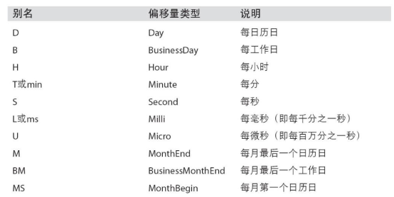
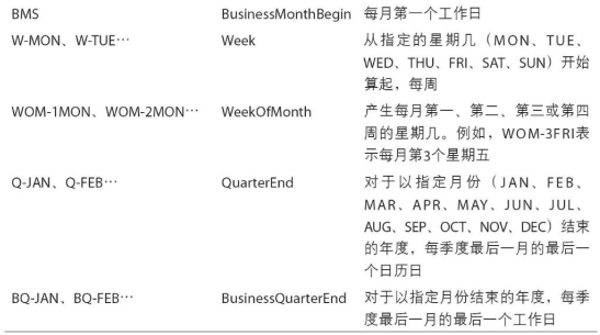
- 偏移量,每个基础频率对应一个偏移量
1.偏移量通过加法连接
sum_offset = pd.tseries.offsets.Week(2) + pd.tseries.offsets.Hour(12)
print(sum_offset)

print(pd.date_range('2017/02/18','2017/03/18',freq=sum_offset))
14 days 12:00:00
DatetimeIndex(['2017-02-18 00:00:00','2017-03-04 12:00:00'],freq='348H')
移动数据
沿时间轴将数据前移或后移,保持索引不变
ts = pd.Series(np.random.randn(5),index=pd.date_range('20170218',periods=5,freq='W-SAT'))
print(ts)
2017-02-18   -0.208622
2017-02-25    0.616093
2017-03-04   -0.424725
2017-03-11   -0.361475
2017-03-18    0.761274
Freq: W-SAT,dtype: float64
向后移动一位:print(ts.shift(1))
2017-02-18         NaN
2017-02-25   -0.208622
2017-03-04    0.616093
2017-03-11   -0.424725
2017-03-18   -0.361475
Freq: W-SAT,dtype: float64
pd.to_datetime()
import pandas as pd
s_obj = pd.Series(['2017/02/18','2017/02/19','2017-02-26'],name='course_time')
s_obj2 = pd.to_datetime(s_obj)
print(s_obj2)
0 2017-02-18
1 2017-02-19
2 2017-02-25
3 2017-02-26
Name: course_time,dtype: datetime64[ns]
# 处理缺失值
s_obj3 = pd.Series(['2017/02/18','2017-02-26'] + [None],name='course_time')
print(s_obj3)
0    2017/02/18
1    2017/02/19
2    2017-02-25
3    2017-02-26
4          None
Name: course_time,dtype: object
时间周期计算
- Period 类,通过字符串或整数及基础频率构造
- Period 对象可进行数学运算,但要保证具有相同的基础频率
- period_range,创建指定规则的时间周期范围,生成 Periodlndex 索引,可用于创建 Series 或 DataFrame
- 时间周期的频率转换,asfreq
- 如:年度周期->月度周期
- 按季度计算时间周期频率
2.2 时间数据重采样
重采样(resampling)
- 将时间序列从一个频率转换到另一个频率的过程,需要
聚合 - 高频率->低频率,downsampling,相反为 upsampling
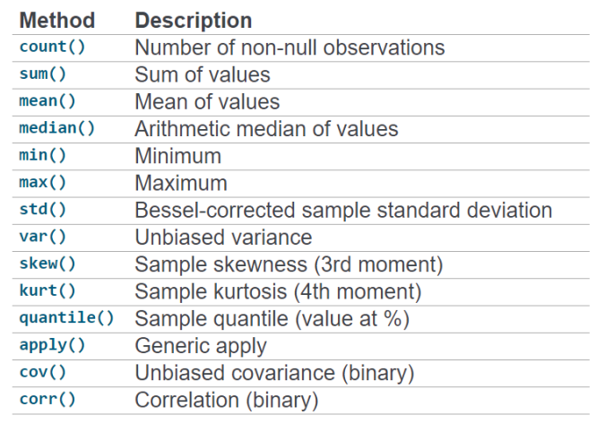
- pandas 中的 resample 方法实现重采样
- 产生 Resampler 对象
- reample(freq).sum0,resampe(freq).mean).…
import pandas as pd
import numpy as np

date_rng = pd.date_range('20170101',periods=100,freq='D')
ser_obj = pd.Series(range(len(date_rng)),index=date_rng)

# 统计每个月的数据总和
resample_month_sum = ser_obj.resample('M').sum()
# 统计每个月的数据平均
resample_month_mean = ser_obj.resample('M').mean()

print('按月求和:',resample_month_sum)
print('按月求均值:',resample_month_mean)
按月求和: 2017-01-31     465
2017-02-28    1246
2017-03-31    2294
2017-04-30     945
Freq: M,dtype: int32
按月求均值: 2017-01-31    15.0
2017-02-28    44.5
2017-03-31    74.0
2017-04-30    94.5
Freq: M,dtype: float64
降采样(downsampling)
- 将数据聚合到规整的低频率
- OHLC重采样,open,high,low,close
# 将数据聚合到5天的频率
five_day_sum_sample = ser_obj.resample('5D').sum()
five_day_mean_sample = ser_obj.resample('5D').mean()
five_day_ohlc_sample = ser_obj.resample('5D').ohlc()
- 使用 groupby 降采样
使用函数对其进行分组操作ser_obj.groupby(lambda x: x.month).sum()ser_obj.groupby(lambda x: x.weekday).sum()
升采样(upsampling)
- 将数据从低频转到高频,需要
插值,否则为 NaN (直接重采样会产生空值) - 常用的插值方法
- ffill(limit),空值取前面的值填充,limit 为填充个数
df.resample(‘D‘).ffill(2) - bfill(limit),空值取后面的值填充
df.resample(‘D‘).bfill() - fillna(fill‘)或 fllna(‘bfill)
df.resample(‘D‘).fillna(‘ffill‘) - interpolate,根据插值算法补全数据
线性算法:df.resample(‘D‘).interpolate(‘linear‘)
具体可以参考:pandas.core.resample.Resampler.interpolate
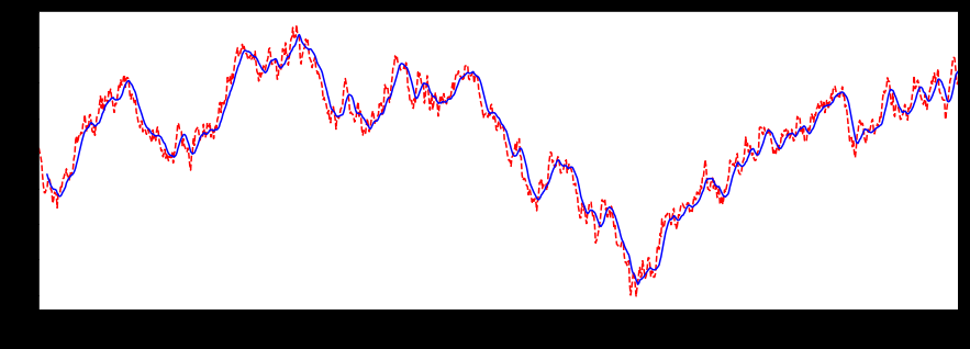
2.3 滑动窗口
- 窗口函数(window functions)
- 滚动统计(rolling)
obj.rolling().func
import pandas as pd
import numpy as np

ser_obj = pd.Series(np.random.randn(1000),index=pd.date_range('20170101',periods=1000))
ser_obj = ser_obj.cumsum()
r_obj = ser_obj.rolling(window=5)
print(r_obj)
Rolling [window=5,center=False,axis=0]
- window
窗口大小 - center
窗口是否居中统计
设置居中:
# 画图查看
import matplotlib.pyplot as plt
%matplotlib inline

plt.figure(figsize=(15,5))

ser_obj.plot(style='r--')
ser_obj.rolling(window=10,center=True).mean().plot(style='b')
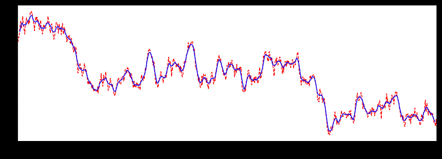
不设置居中:ser_obj.rolling(window=10,center=False).mean().plot(style=‘b‘)

版权声明:本文内容由互联网用户自发贡献,该文观点与技术仅代表作者本人。本站仅提供信息存储空间服务,不拥有所有权,不承担相关法律责任。如发现本站有涉嫌侵权/违法违规的内容, 请发送邮件至 dio@foxmail.com 举报,一经查实,本站将立刻删除。

